Topic 11- Radiation Dosimetry
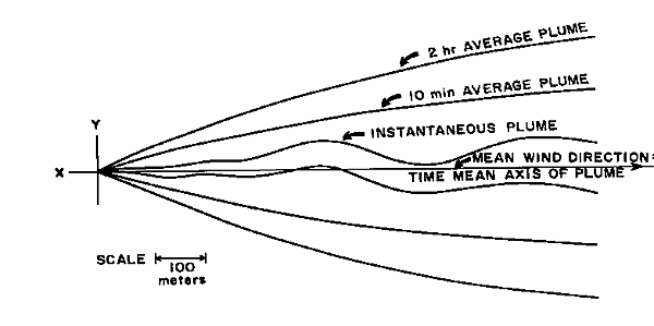
Gaussian Plume Model |
 |
 |
Studies at the Surface Friction Layer

- C = concentration
- Q = source strength
- sz sy
= crosswind & vertical plume standard deviations
-
 = mean wind speedF
- h = effective stack height
- x, y = downwind and crosswind distances
- z = height above ground
- This calculates the concentration downwind of gases & particles
with negligible settling velocity (< 20µm)
Gaussian Plume Model

- Used to describe ground-level concentration downwind from a continuously
emitting point source:
- C = concentration
- Q = source strength
- sz sy
= crosswind & vertical plume standard deviations
-
= mean wind speed
- h = effective stack height
- x, y = downwind and crosswind distances
Numerical Values for Lateral Diffusion (sy)

Numerical Values for Vertical Diffusion (sz)

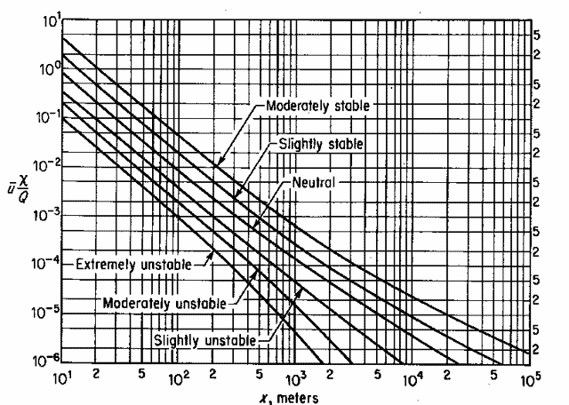
Normalized Equations Ground Level
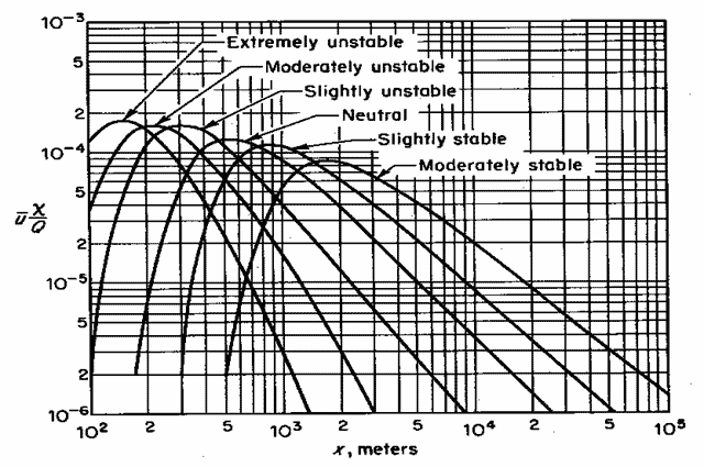
Normalized Equations 30 m Stack
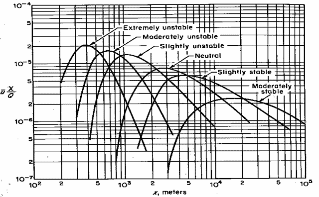
Normalized Equations, 100 m Stack
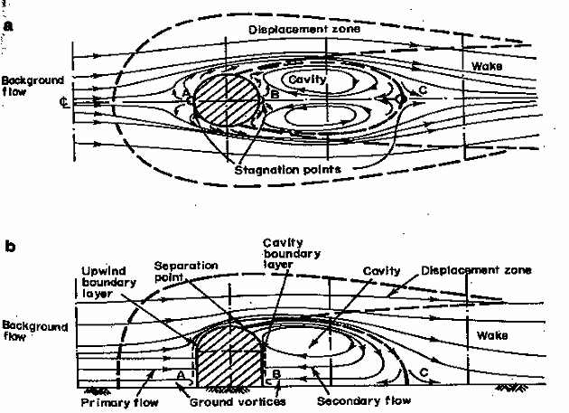
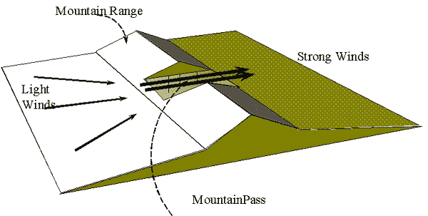
Effects of Buildings on Plume Dispersion
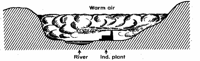
Effects of Terrain on Plume Dispersion


Presenting Wind Data
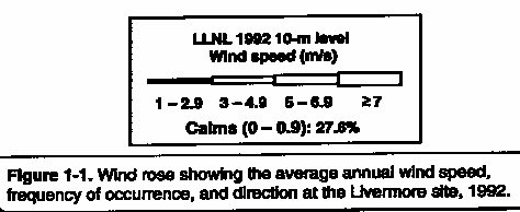
Recording Wind Data
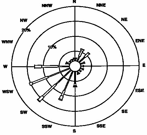
| |
Livermore site |
| Direction |
Calm
0.0-0.9 |
1.0-2.9 |
3.0-4.9 |
5.0-6.9 |
>7.0 |
Total |
| N |
1.7 |
0.4 |
0.3 |
0.3 |
0.1 |
2.8 |
| NNE |
1.7 |
1.8 |
2.0 |
0.5 |
0.1 |
6.1 |
| NE |
1.7 |
2.5 |
1.7 |
0.1 |
0.0 |
6.0 |
| ENE |
1.7 |
1.3 |
0.2 |
0.0 |
0.0 |
3.2 |
| E |
1.7 |
0.9 |
0.1 |
0.0 |
0.0 |
2.7 |
| ESE |
1.7 |
1.1 |
0.0 |
0.0 |
0.0 |
2.8 |
| SE |
1.7 |
0.7 |
0.1 |
0.0 |
0.0 |
2.5 |
| SSE |
1.7 |
0.8 |
0.3 |
0.0 |
0.0 |
2.8 |
| S |
1.7 |
4.1 |
0.7 |
0.3 |
0.2 |
7.0 |
| SSW |
1.7 |
7.0 |
2.0 |
1.2 |
0.3 |
12.2 |
| SW |
1.7 |
6.8 |
5.6 |
1.8 |
0.2 |
16.1 |
| WSW |
1.7 |
7.4 |
5.3 |
0.9 |
0.0 |
15.3 |
| W |
1.7 |
3.6 |
5.1 |
2.2 |
0.1 |
12.7 |
| WNW |
1.7 |
0.9 |
0.3 |
0.0 |
0.0 |
2.9 |
| NW |
1.7 |
0.6 |
0.1 |
0.1 |
0.0 |
2.4 |
| NNW |
1.7 |
0.6 |
0.1 |
0.1 |
0.0 |
2.5 |
| Total |
27.2 |
40.4 |
23.9 |
7.4 |
1.0 |
100.0 |
Computer Models for Atmospheric Calculations
- Computer codes are preferred method
- AIRDOS
- CAP88
- COMPLY
- ISCLT
- TRAC
- MESODIF
- Gaussian Plume Model
- Puff Trajectory Model
- Other
Troposhperic and Stratospheric Behavior
- Previously discussed near surface emissions
- Diffusion over tens to hundreds of kilometers
- Beyond that no interest for industrial or research
- Nuclear explosions or major violent accidents are different
- Chernobyl spread globally
Meridional transport
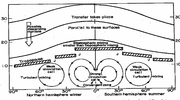
Tropospheric and Stratospheric Behavior
- Residence of stratospheric aerosols depends on
- Altitude
- Time of year
- Latitude dependent
- Russian explosions into stratosphere had mean residence time of <
6 mo
- Explosions into mid stratosphere in tropics had 2-3 year residence
- But, 5-10 y at 100 km elevation
Transport in Troposphere and Stratosphere
- Aerosols introduced into troposphere are distributed by planetary
winds
- Deposited by rain scavenging
- Example, 90Sr and rainfall
- Mean residence time of dust is ~ 30 days
- Rainfall removes particles primarily by rainout (droplet formation
around the particle)
- Ocean spray scavenging may be a factor
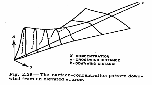
Elevated Releases - Qualitative
Characterizing Turbulent Diffusion
- Gradient Transport Theory
- transport at a fixed point
- similar to molecular diffusion
- Statistical Theory
- study history of motion
- determine statistical properties needed to represent diffusion
- For large diffusion times, both generate the Gaussian distribution
Instantaneous Releases

- Explosion or puff
- Puff diffuses in 3 dimensions
- Formula estimates ground-level air concentrations downwind
- Where
- QT = total quantity of material released
- sx,y,z standard
deviation of puffs
- u, mean wind speed
- t = time in sec after release
Gaussian Diffusion of Single Puffs

Predictive equations for Diffusion Values Between 100 and 4000 m
| Parameter (m) |
Stability Class |
Power Function |
| sy |
Unstable |
0.14X0.92 |
| Neutral |
0.06X0.92 |
| Very Stable |
0.02X0.92 |
| sz |
Unstable |
0.53X0.92 |
| Neutral |
0.15X0.92 |
| Very Stable |
0.04X0.92 |
| s'x
is presumed to behave as s'y |
Continuous Releases, Infinite Number of Clouds

Gaussian Plume Diffusion

Gaussian Plume, Reflection at Surface

Long-term average air concentrations
- At a given point
- Must account for changes in
- wind speed
- win direction
- atmospheric stability

Seasonal concentration Calculations
- Avoids use of sz
- Requires frequency of each stability class
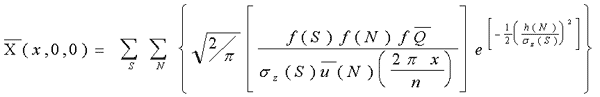
- Where
- f(S) = frequency of stability class S
- f(N) = frequency wind speed class N
- f = frequency of wind in sector
- sz(S) = vertical
dispersion class S
- u(N) = mean wind speed for class N
Prerequisites and Assumptions
- Model is valid assuming:
- Homogeneity of turbulence
- Requires uniformity of topography
- Stationary turbulence
- Requires transport in= transport out
- (I.E. Source & turbulence constant)
- Valid for hours at a time
- Long diffusion times
- Spatially constant basic flow
- Wind velocity unchanged with height
- OK up to ~ 150 m
Stationary Diffusion
Effect of Diffusion Times
Assumptions, Continued
- Nonzero wind speed
- Need to neglect diffusion in x direction
- Or use Gaussian puff model
- Total reflection of the plume
- Ignore ground deposition (depletion)
- Conservative approach
Practical Consequences of Using Gaussian Plume
- Theoretical assumptions, etc rarely met
- Empirical studies of diffusion parameters make model predictions
~ reasonable
- Allows model to be used for estimating long periods, varying turbulent
states
Diffusion Parameters
- Model expressed in terms of sy
sz
- Selection of appropriate values subjective & controversial
- Major tests done to determine parameters, variety of tracers (radioactive
and stable)
- Several parameter systems defined for short term, long term, ground
level, etc
- All have some relevance
- Be careful
Practical Applications of Gaussian Plume
- C (Ci/m3) - limited use
- Need normalized, time-integrated air concentration
- E(Ci-s/m3): estimates dose in ith sector
- Inhalation
- Submersion
- Total deposition

Sector Averaged Calculations
- N = total probability of wind in all frequencies, stabilities, &
class (i.e., 100%)
- k = wind speed in class k
- j = stability in class j
- njk = percentage of time of occurrence of wind direction(i),
speed(k), and stability class (j)
- k
= representative windspeed in class k
- szj = diffusion
parameter for stability class j
- x = downwind distance
- For n=16 sectors
Atmospheric Transport, Continued
- Dispersion of aerosols vs gases
- Plume depletion and enhancement mechanisms
- Tropospheric and stratospheric behavior
Gaussian Plume Model
- Advantages
- Simple
- Can be hand calculated
- Limitations
- Flat terrain
- Predictions valid within factor of 2 -3
- Valid only to 10 km downwind
- Cannot account for curvature in wind direction
- Much less valid for complex terrain
Plume Enhancement & Depletion Mechanisms
- Depletion mechanisms
- Dry deposition
- Gravitational settling
- Impaction
- Washout
- Precipitation washes dust from air
- Rainout
- Dust serves as condensation nuclei
- Process removes most submicron particles from atmosphere
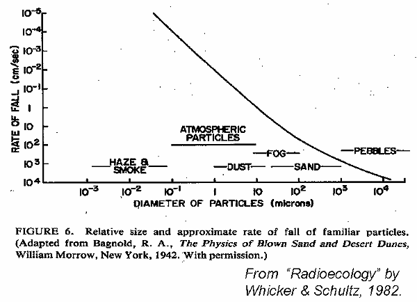
Particles
- What are they?
- Distinct portion of solid , liquid, or gas larger than single
molecule
- Size classification based on how particles are measured (e.g., Sieve
sizes, settling velocities ..)
- Classifications
- Based on media
- Colloids - 1 to 400 nm
- Solids dispersed in gas - smoke/aerosol
- Liquids in gas - fog, aerosol
Properties of Colloids
- Enhanced adsorption
- Ability to concentrate substances on their surfaces)
- Large surface area to volume ratio
- Electric charge (positive or negative)
- Described by concentration
- Mass particulate/m3
- Mass particulate/m2
- Activity/m3
- Activity/m2
Particle Sizes & Rates of Fall
Gravitational Settling
- Falling particle accelerates with gravity until constant velocity
reached
- Terminal velocity balance of
- Resistance offered by fluid medium (acts opposite to weight of
particle)
- Radius/density determine weight & downward force
- Opposing (aerodynamic drag) f(size, velocity, density, viscosity,
resistance to sheer stress)
Gravitational Settling of Particles
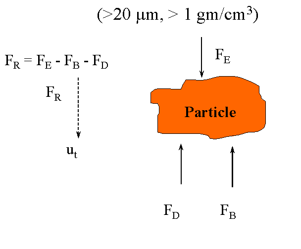
Gravitational Settling
- Applicable to particles in fluid or air
- FR = resultant force on particle
- FE = external force on particle (e.G., Gravity or centrifugal
force)
- FB = buoyancy force
- FD= friction or drag force, opposing settling of particle
- ut = terminal settling velocity
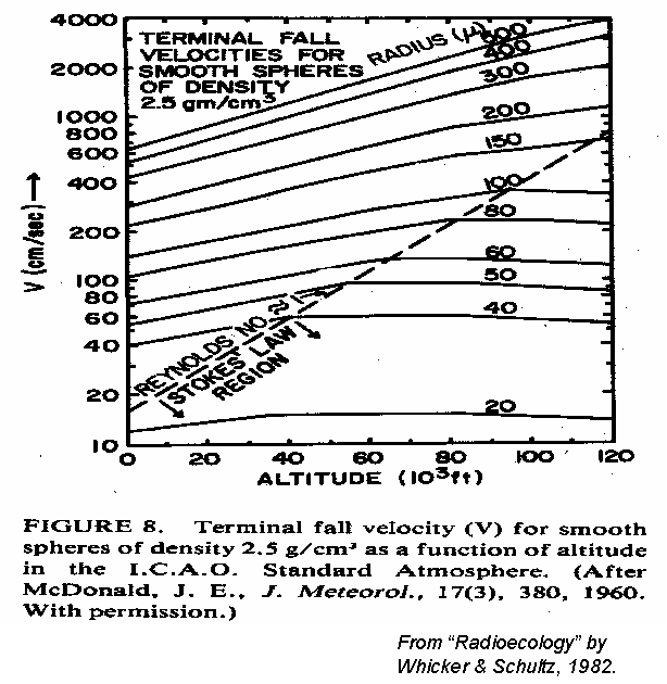
Particle Gravitational Settling

- Assumptions
- spherical particle
- terminal velocity (ut)
- laminar flow
- rp = density
of particle
- r = density of air
- g = gravitational settling
- d = particle diameter
- µm = absolute viscosity of air
Terminal Fall Velocity for Smooth Spheres
Particle Settling - Dry Deposition
- <20 µm particle size or gases
- Deposit at rates > gravitational settling
- Other mechanisms responsible:
- Surface impaction
- Electrostatic attraction
- Adsorption
- Chemical interaction
- Determined experimentally as ratio between deposition and air concentration
Dry Deposition
- Deposition velocity:
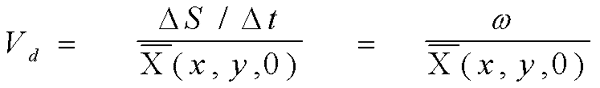
- Vd , deposition velocity, m/s
- DS = mass of particles per
unit of surface area (g/m2)
- Dt = time increment (s)
- C = mean ground level air concentration (g/m3)
- w = deposition rate (g/m2-s)
Deposition Velocities
- Empirical approach acceptable
- Loss mechanisms ignored or accounted for
- Experiment period is short
- Vd is dependent upon
- Particle size
- Particle density
- Shape
- Electrostatic charge
- Surface chemistry
Deposition Velocities, continued
- Surface parameters of importance include:
- Texture
- Roughness
- Presence of hairs or other projections
- Electrostatic charge
- Surface chemistry
- Effective surface area
- Surface orientation
Deposition Velocity Values
- Extremely variable
- Five orders of magnitude range for dusts (10-3 - 10-8
cm/s)
- Less variability for gases
- 2 cm/s for reactive iodine on grasses
- 0.1 cm/s for particles less than 4 µm
- 0.018 cm/s for unreactive gases
Deposition Velocity Caveats
- This is not a true velocity;
- A measure of dry removal processes
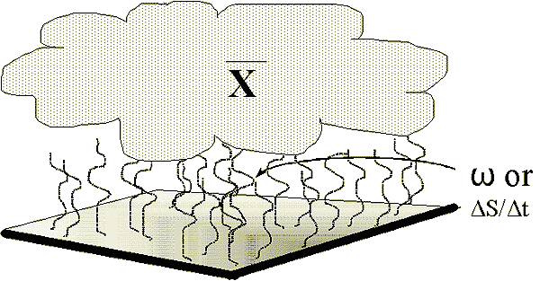
Wet Deposition
- Rain and snowfall - precipitation scavenging
- Rainout (in-cloud scavenging)
- Can involve submicron particles
- Washout
- Below cloud scavenging
- Effective for particles >1µm

- Lamda = washout coefficient
- Lamda = 1.6 x 10⁻⁴rp0.8
- Rp= rainfall rate, mm/h
Washout Coefficients
Cloud Depletion From Washout
- x = downwind distance, m
- u = mean wind speed acting on the plume
- (From whicker & Schultz, radioecology, 1982)
Plume Enhancement Mechanisms
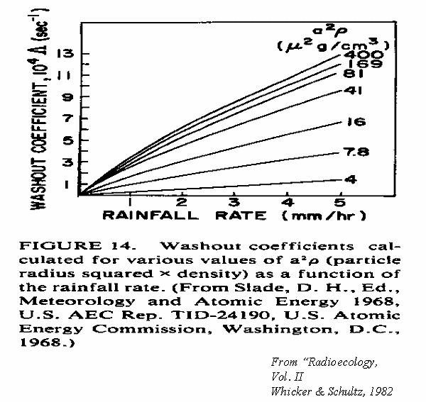
- Resuspension
- Small particles (< 50µm) elevated from ground surface
- Subset of wind erosion
- Atmospheric variables include
- Velocity
- Turbulence
- Density = f(temp, press., Humid.)
- Viscosity
Plume Enhancement Mechanisms
- Soil variables include:
- Texture (particle size distribution)
- Cohesiveness
- Moisture content
- Density
- Plant cover
- Ground surface roughness
- Topography
Soil Sizes and Erodibility
| Principle Transport Mechanism |
Particle Diameter (µm) |
Relative Erodibility |
| Airborne Transport |
< 20 |
Nonerodible, except at very high wind speeds |
| 20 - 50 |
Difficultly erodible |
| Saltation |
50 - 500 |
Highly erodible |
| 500 - 1000 |
Difficultly erodible |
| Surface Creep |
> 1000 |
Nonerodible except at high wind speeds |
Resuspension Mechanisms
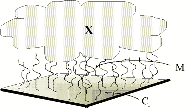
Approaches to Estimating Resuspension
- Mass loading
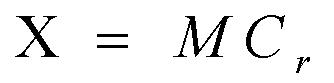
- X = air concentration in µCi/m3
- M = air dust load in g/m3
- Cr = concentration in the resuspendable fraction
of the soil in µCi/g
Mass-loading
Resuspension Factor
- Alternative to Mass Loading
- R = X/S
- R = resuspension factor, m-1
- X = air concentration, µCi/m3
- S = surface deposition, µCi/m2
Caveats on Plume Depletion/Enhancement
- Extreme variability in ranges
- Multiple approaches available
- Variety of physical processes influence
- Site specific parameters may be developed based on experiments
Atmospheric Model Recap
- Generally conservative
- Tend to over predict concentration
- Under predict plume spread
- Model accuracy limited to factor of 2 at best
- Complex dispersion models
- More physically realistic treatment
- Limited predictive improvement
- But they cost more and are more time consuming
|